Signal Integrity Constraints

This is Part 2 of the Signal Integrity Essentials series. Part 1 on Topologies provides a lot of background information you may find useful before proceeding with this section.

The topology provides the geometry framework upon which more advanced constraints are applied. It allows for these more advanced constraints to be easily specified. Typically, this means specifying the "endpoints" of a topology. The routing engine will infer the nodes between those two endpoints and apply the constraint on all segments and nodes between the endpoints.

Constraints

Constraints come in the form:

1. Medium Independent Constraints - For example, Routing Structures encode the properties of the physical medium to create impedance controlled geometry. These are applied with the structure statement.
2. Medium Dependent Constraints - These constraints require a valid Routing Structure constraint.
   1. Timing - These encode the limits on the delay of the signal through the medium.
   2. Timing Difference - These encode the limits of the difference in signal delay between two signals.
   3. Insertion Loss - These encode the limits on the loss of the signal through the medium.

Medium Independent Constraints

The medium constraints are primarily geometric constructs that define how a transmission line is formed in the PCB. These provide the broad class of controlled impedance constraints. In addition to geometry, these constraints will often provide necessary data to characterize the PCB transmission medium. These characteristics, like propagation speed, loss, etc, are used by other constraints.

One example of the medium constraints is the Routing Structures. In the current JITX runtime, these come in a "single-ended" and "differential" forms. This allows the user the opportunity to construct transmission lines like:

• Microstrips
• Striplines
• Edge-Coupled Striplines
• And many others.

NeckDown & Structures

The routing structures all provide a Neckdown configuration. The goal of neckdown is to provided an automated and constraint-based mechanism for the fan-out or fan-in of an impedance controlled signal. Often times in BGAs or other space constrainted packages, the terminations for impedance controlled signals may have narrow spacing. This may violate the typical clearance requirements that we want for our signal. The neckdown provides a way to specify the features of the trace in these areas of the board.

Time-based Constraints

Users familiar with legacy CAD systems will be familiar with the concepts of "Length Matching." This is a very intuitive way to think about the propagation of signals. If the length of two signals are the same, then surely the propagation of the signals through the transmission line will be the same. This approximation leaves out of its analysis much of the nuance in high speed circuit design. The propagation delay for a signal through a particular medium is dependent on several factors. Transitioning from a top side microstrip to an internal stripline introduces yet more diversity in the propagation delay.

The problem with the length is that there isn't really a way to modulate it given the physical characteristics of the medium. You could make arbitrary scaling factors on the length to account for things like vias, stripline vs microstrip, etc, but at the end of the day, these are all just fudge factors. There is no way to align these with the results from a simulation system like HFSS or Keysight ADS.

The routing structure constraints provide a mechanism to formulate the signal propagation delay for signals on different layers and through other structures. The routing engine can use this information to compute the delays or losses and then optimize the route geometry to meet the applied constraints.

Timing Constraint

The timing constraint is a mechanism for explicitly controlling the delay of a given signal.

A signal propagates from the source to the destination, starting at time t0 and arriving at the receiver at t1. The delay for the signal is t1 - t0. This constraint type sets the limits for this delay.

This functionality is not super common but is useful for many RF applications - like phased array antennas.

  val phase-delay = 1.0e-9 +/- 10.0e-12
  timing(elem[0], elem[1]) = TimingConstraint(phase-delay)

In this example, we establish an element to element phase delay of 1.0ns ± 10ps. The timing statement works on the "endpoints" of the topology. These endpoints typically resolve to the pads of the component (in this case, the feed pad of the patch antenna element).

Once the trace with a timing constraint is realized, the constraint will force the routing engine to continuously evaluate the characteristics of the trace. You will see a message in the "Issues List" under "Unsatisfied Signal Constraints":

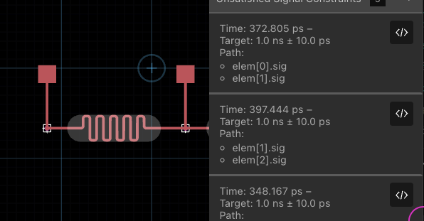
1. The "Time" meaning the current delay of the signal as calculated by the routing engine.
2. The "Target" meaning the actual constraint we're trying to achieve, in this case 1.0ns ± 10ps.
3. The "Path" meaning the endpoints that identify the path on the topology where this constraint is applied.

The shaded section is a "Signal Tuning" section (previously called the "Length Matching" section). Inside this section, the routing engine attempts to match the tuning parameters, primarily delay and loss, to meet the constraint requirements. In the above example, the signal tuning section is too small. So the routing engine makes its best effort and packs the signal tuning section with as many squiggle periods as it can. It then creates the "Unsatisfied Signal Constraint" issue in the issues list.

If the signal tuning section is large enough, the routing engine will typically optimize the length of the trace with variable pitch and amplitude of the "squiggle." Here are some examples of how the routing engine might create this trace in this case:

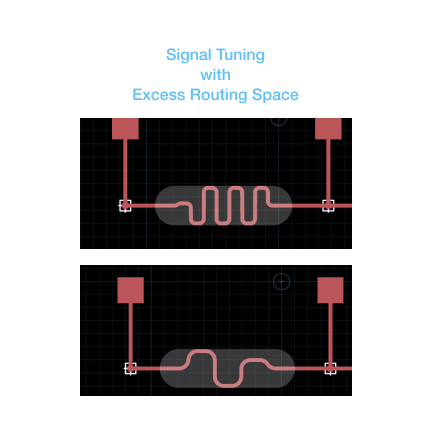
In this example, I've changed the signal propagation speed to slow down the signal artificially. This allows the routing engine some breathing room to demonstrate the above cases.

Notice that the period of squiggle changes and eventually the amplitude. The size of the signal tuning region defines the maximum amplitude of the signal. Currently, the other parameters of the squiggle like mininum turn radius, minimum period, and shape are not controllable by the user, but these will come in the future.

When the signal successfully achieves the timing constraint - the "Unsatisfied Signal Constraint" issue will disappear from the list. This is an actively assessed condition and changes in the board may cause it to re-appear.

Caution: Currently, vias are modeled with a constant delay/loss model. Future versions of JITX will provide customization of via delay. If the signal enters and exits on the same layer - no delay or loss is introduced. If the signal enters and exits on different layers - then a 20pS delay and a 0.15dB loss are introduced.

Timing Difference Constraint

The timing-difference constraint introduces a mechanism for controlling the timing skew between two signals.

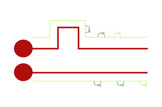
Two signals propagate down a transmission line and at the end there is a time difference or skew between the two signals (shown below as ∆T):

This is a very common constraint in a wide variety of applications:

1. Differential Pairs
   1. Intra-pair skew - ie, P to N.
   2. Inter-pair skew - for example, in MIPI-CSI for CLK and DATA diff-pair lanes.
2. Parallel Data Buses
   1. Bus Member to Member
   2. Bus Members to Strobe, for example in DDR memory

For "intra-pair" skew, the timing difference constraint drives the routing engine to use deskew bumps in the "Signal Tuning" regions. These "deskew bumps" attempt to achieve a phase matched relationship between the P and N signals of a differential pair.

Here is an example with differential pairs and timing-difference for intra-pair and inter-pair constraints:

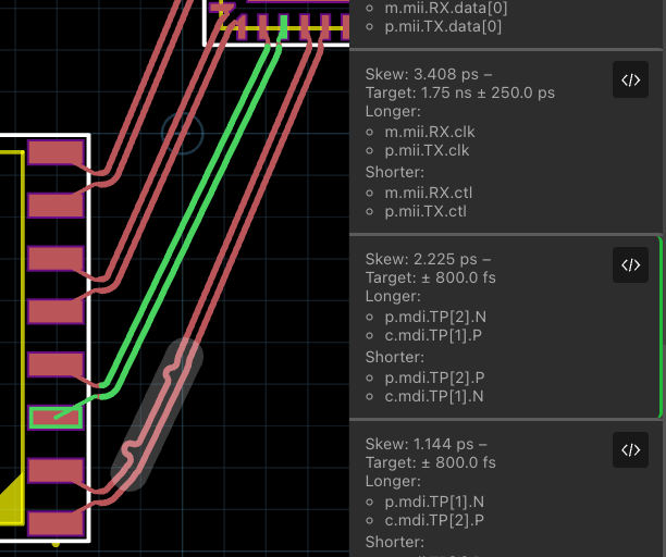
In the image above we can see multiple differential pairs routed in a circuit. The "Issues List" on the left shows the current set of "Unsatisfied Signal Constraints." In this case, we have selected the first intra-pair skew constraint that is unsatisfied. The board view shows the associated traces highlighted in the board view. It is displaying for useful information for diagnosing and resolving this constraint:

1. The Skew is the current total skew between the signals in this diff-pair bundle signal.
2. The Target is the constraint specified in code. In this case we're targeting 0.0 ± 800.0 fs (femtoseconds).
   1. This constraint is likely more restrictive than you will see in practice.
   2. We've exaggerated this constraint to make it easier to demonstrate this matching condition in JITX.
3. Longer and Shorter refer to the delay of the compared signal topologies by endpoint.
   1. In this particular example, the PHY side allows for swapping P and N in the diff-pair.
   2. Hovering over the longer or shorter endpoints will highlight those routes on the board.

Beside that differential pair is another differential pair with a signal tuning section applied to it. Notice in that in this signal tuning section, the routing engine has applied two deskewing bumps of different sizes. Notice that the maximum amplitude of the deskew bumps is defined by the signal tuning sections envelope and a hard-coded maximum bump amplitude. The routing engine constructs these deskew bumps to remove the skew between the P and N signals per the user's constraints.

Deskew Bump Features

Creating useful deskew bumps is a complex task. There are many knobs and features to tweak to get a reasonable circuit representation. The following section is going to outline some of these features. Keep in mind that in the current implementation, many of these features are hard-coded. Future JITX versions will make more of these features accessible for configuration.

Deskew Bump Amplitude

As described above, the amplitude for the deskew bumps is defined by the envelope of the signal tuning region. But depending on conditions, the routing engine will attempt to maximize what area it has available to it.

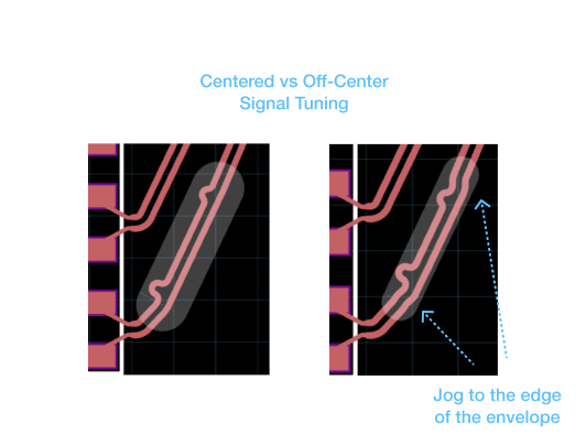
In the example above, if we oversize the envelope, then the differential pair will center itself to take the shortest path. If the envelope is too small, then the router will attempt to shove the differential pair as far to one side as it can in order to maximize the deskew bump amplitude.

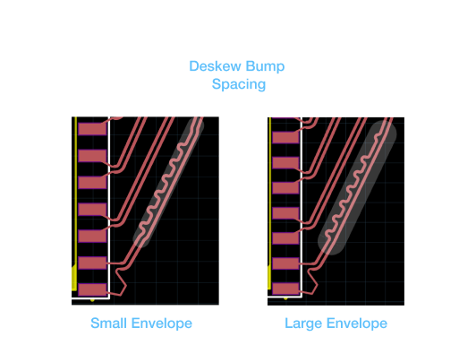
Deskew Bump Spacing

The spacing between deskew bumps is typically a Notice that that the deskew bumps are spaced according to the size of the envelope. In addition, the algorithm is currently hard coded with a maximum space between deskew bumps within a given envelope.

Power-based Constraints

A common first order approximation of loss is the length of the signal. Like with time vs length, this approximation doesn't take into account many of the non-obvious features of a board. The routing engine uses loss as a metric so that we can implement features similar to a channel operating margin analysis.

Insertion Loss Constraint

The insertion-loss constraint provides a mechanism to enforce limits on signal loss. It is common for protocols like USB, PCIe, etc to limit the acceptable insertion loss presented by the PCB.

The most typical application of insertion-loss is to implement a maximum loss restriction on the signal. This constraint depends on a valid routing structure that provides an accurate insertion loss rate for each layer and structure. Without accurate data, this constraint won't be successfully computed.

   val max-loss = InsertionLossConstraint(
    min-max(0.0, 12.0)
  )

  insertion-loss(MCU.micro-sd.CLK => conn.micro-sd.CLK) = max-loss
  ...

The insertion-loss is specified in dB at the frequency of interest. Note that the insertion-loss of the pcb-routing-structure is assumed to be in dB/mm at this same frequency of interest.

Usage Patterns

In the next section, we're going to introduce higher level functions that use the topology and constraint primitives for effective modular designs.