Design Constraints#
JITX’s system of design constraints allows you to control details of physical design such as trace width, clearance, via fencing patterns, thermals, and more, using a general, flexible code-based interface.
Key concepts#
Before diving into examples, here are the four core concepts of the constraint system:
Tag: A label that can be applied to design objects (currently nets). Tags come in two flavors: user tags that you define in code (e.g.
Power,HighSpeed) and implicit tags that the system applies automatically based on an object’s type or layer (e.g.IsTrace,OnLayer(0)). SeeTagandBuiltinTag.Condition: A boolean expression of tags that determines when a constraint applies. Tags can be combined with
&(and),|(or), and~(not). For example,IsTrace & Power() & OnLayer(0)matches traces on the top layer that belong to a power net. SeeBoolExpr.Effect: What a constraint does when its condition is satisfied — for example, setting a trace width or a clearance value. See Effects for the full list.
Constraint: The combination of one or two conditions with one or more effects. Created using the
design_constraintfunction. A constraint with one condition is unary (e.g. trace width); a constraint with two conditions is binary (e.g. clearance between two objects).
When multiple constraints could apply to the same object, JITX uses a constraint selection algorithm based on logical specificity to choose the most relevant one — more specific conditions take precedence over general ones.
Basic usage#
Here is an example of a design constraint:
design_constraint(IsTrace & MyTag() & OnLayer(0)).trace_width(1.0)
This constraint effectively says: whenever a trace on the top layer of the
board has MyTag, set its trace width to 1mm.
Anatomy of a design constraint#
Following this example, let’s take a closer look at the parts of a constraint.
design_constraintis a generic function for defining constraints. It is a convenience wrapper which constructs either aUnaryDesignConstraintor aBinaryDesignConstraintdepending on whether one or two conditions are given. The example is a unary constraint, with one condition and one effect.The first argument of
design_constrainthere,IsTrace & MyTag() & OnLayer(0), is the condition of the constraint. A condition is a boolean expression of tags. The tags here are:MyTag()is a user tag. We must define it ourselves and assign it to objects usingassign.IsTraceandOnLayer(0)are implicit tags. They are pre-defined to apply in particular well-defined circumstances.IsTracemeans the object is a trace andOnLayer(0)means it is on the top layer of the board.
trace_width(1.0)is the effect of the constraint. When the condition is satisfied, assuming no other constraint takes precedence, this effect describes what the constraint will actually do to the design.
Using the constraint in a design#
In order to use this constraint, a few more bits of code are needed. The following is a simplified sketch — a complete design would also include components with pads connected to the nets, a board outline, and a substrate definition.
# define our tag
class MyTag(Tag):
  pass

class MyCircuit(Circuit):
  my_special_net = Net()
  my_other_special_net = Net()

  def __init__(self):
      # Assign our tag to some nets so that the constraint
      # will apply to their physical objects.
      MyTag().assign(self.my_special_net,
                     self.my_other_special_net)

class MyDesign(Design):
  board = MyBoard()
  substrate = MySubstrate()
  circuit = MyCircuit()

  def __init__(self):
    # Trace width for tagged traces on the top layer
    self.tw = design_constraint(
        IsTrace & MyTag() & OnLayer(0)
    ).trace_width(1.0)

    # Clearance constraints for tagged copper
    self.clr = [
      design_constraint(
          IsCopper & MyTag(), IsCopper
      ).clearance(0.7),
      design_constraint(
          IsCopper & MyTag(), IsBoardEdge
      ).clearance(2.0),
    ]
Notice in this example all the ingredients to make a constraint actually take effect in the design:
Define a tag by defining a new class which inherits from
Tag.Define a constraint using the tag.
Put the constraint inside any design object by assigning it to
self. Constraints can be added anywhere in the design tree (in aDesign, aCircuit, or any sub-circuit). See the documentation on circuits for more details on how to add objects to designs.
Conditions#
Constraint conditions are boolean expressions of
tags. That means tags can be combined using the boolean operators &, |, and
~ (“and”, “or”, and “not”, respectively, also known as conjunction,
disjunction, and negation). Conditions determine to which objects the
constraint effects will be applied. Each object will have a list of tags, and a
condition applies if it logically evaluates to true for that set of tags when we
treat each tag inside the condition as true if the object has it, and false
otherwise.
A constraint may have one or two conditions — the number of conditions is called the arity of the constraint. All constraints currently used in JITX have either 1 condition or 2 conditions; these are called unary and binary constraints, respectively. The effects of a constraint must match the arity of the conditions; a unary effect is something which applies to a single object and a binary effect applies to a pair of objects. Currently the only binary effect type is clearance.
The special constant AnyObject matches any
object regardless of its tags. It is useful when one side of a binary
constraint should apply universally:
design_constraint(IsTrace & HighSpeed(), AnyObject).clearance(2.0)
Like tags, expressions are full-fledged objects in their own right and can be defined and manipulated by utilities to make constraints easier to write. For example:
any_inner = ~(OnLayer(0) | OnLayer(-1))
power_other = Power() & ~Power3V()
self.dc = design_constraint(IsPour & any_inner,
                            IsTrace & power_other).clearance(1.5)
Conditions are significant not only in determining to which objects a condition may be applied, but also in determining which constraint is considered to take precedence when more than one constraint’s condition applies. See the constraint selection algorithm for details. However, the algorithm still only considers the logical truth function of the condition, and not any other details. For example, these expressions are absolutely equivalent for all purposes:
A | BB | A~(~A & ~B)
Effects#
Each constraint can have one or more effects. Because the system always makes queries for one effect type at a time, specifying multiple effects in a single constraint serves only as a shorthand to prevent rewriting an otherwise-identical constraint multiple times. In other words, there is no difference in meaning between writing one constraint with three effects, and splitting those effects between three different constraints each of which has the same condition.
trace_widthspecifies a width for copper traces. It does not apply to any other kind of object.clearancespecifies a minimum spacing between two objects. Constraints with this binary effect are automatically symmetrized so it does not matter in which order the conditions are given. In other words, one object must satisfy one condition and the other object must satisfy the other condition, it doesn’t matter which is which.Caveat: note that for length-matching regions, clearance is applied to the edge of the region, not to the trace itself.
thermal_reliefsets thermal relief parameters for pours. It does not apply to other objects.stitch_viaandfence_viaset implicit via generation patterns for the appropriate kinds of objects.
Note that design constraints as described here control physical properties of copper objects. For signal integrity constraints such as timing, skew matching, and insertion loss, see the SI constraints documentation.
Introduction to constraint selection#
When you have many constraints in your design, it will typically be the case that multiple constraints with the same effect type (such as clearance) are potentially applicable to the same objects. The system needs to choose which one to use. Each time a constraint query is made, internally JITX runs an algorithm to choose which constraint should be applied, among all constraints which supply the relevant effect type.
Let’s walk through an example which shows how you can take advantage of the constraint selection algorithm to override existing constraints in specific cases where you need to. Suppose you are writing constraints to manage your power routing. Your design has this constraint:
design_constraint(IsCopper & Power(), IsCopper).clearance(1.5)
and you have applied this Power tag to the appropriate nets. Now you realize
you need more clearance to vias in particular, so you add another constraint:
design_constraint(IsCopper & Power(), IsVia).clearance(2.0)
Note that both of these constraints are logically applicable whenever a power
route goes near a via (because IsVia inherits from IsCopper). You can
always make certain of which constraint will take precedence by adding an
explicit priority. However, to
streamline constraint writing, the selection algorithm uses a principle of
logical specificity which ensures your new constraint,
the one which specifically applies to vias, will be the one that is applied.
The idea is that without such semantics, there wouldn’t be any reason for the
more specific constraint to exist: IsVia implies IsCopper so if the older
constraint using IsCopper took precedence, the more specific
constraint would never have a chance to do anything. Similarly, if you had a
generic clearance constraint
design_constraint(IsCopper, IsCopper).clearance(0.3)
that would not interfere with the functioning of the power constraints. We should also emphasize that it is not just a question of taking a larger clearance. For example, you might need to relax the power clearance constraint for one net in particular. You can do this with the help of a new tag which inherits from your Power tag like this:
class Power3V(Power):
    pass

design_constraint(IsCopper & Power3V(), IsVia).clearance(1.5)
The specificity principle means that this constraint overrides the above clearance
from Power to IsVia.
Hopefully this is all reasonably intuitive so far, but inevitably you will run into cases that are more ambiguous. For example, suppose you instead made a relaxed constraint for this net to any copper instead of just vias:
design_constraint(IsCopper & Power3V(), IsCopper).clearance(1.0)
Now when the system is computing the clearance from this specific net to a via, all these constraints are logically applicable:
design_constraint(IsCopper, IsCopper).clearance(0.3)             # constraint A
design_constraint(IsCopper & Power(), IsVia).clearance(1.5)      # constraint B
design_constraint(IsCopper & Power3V(), IsCopper).clearance(1.0) # constraint C
Constraint A clearly shouldn’t apply, but it is apparently ambiguous whether
constraint B or C is more specific. B has a more specific object type tag
(IsVia) in the second argument and C has a more specific user tag, (Power3V)
in the first argument. What happens in fact here is that constraint B will be
applied, because specificity in object types is considered to outweigh most
other kinds of specificity. See the canonical tag
ordering for details.
In a case like this, you can use the explicit
priority keyword argument to
the design_constraint function to
remove any doubt about which constraint will take effect. The drawback of this
approach is that you will never again be able to override this constraint except
by another constraint with the same or higher priority - it pre-empts any future
attempt to flesh out more detailed behavior using constraints at the current
priority level. Once you start using explicit priorities, it can become a burden
to maintain what is effectively a manually ordered list of constraints. In this
case, if you want constraint C to apply instead of B, without using explicit
priority, you might simply add a negation to prevent the constraint B from
being considered for Power3V nets:
design_constraint(IsCopper & Power() & ~Power3V(), IsVia).clearance(1.5)
By understanding the selection algorithm, you can take advantage of the specificity principle to write elegant sets of constraints that are easy to maintain and expand.
Overview of algorithm#
A constraint query is run whenever the JITX backend needs a value which can be controlled by constraint effect. For example, whenever the autorouter runs it will make numerous queries about the trace width of various routes and the clearance that they need to other objects, so that correct routes can be chosen and saved. Every new constraint query goes through the constraint selection algorithm, which initially considers all constraints in the design with the appropriate effect type and gradually narrows the set of candidates until just one constraint is chosen. The effect of that constraint is used.
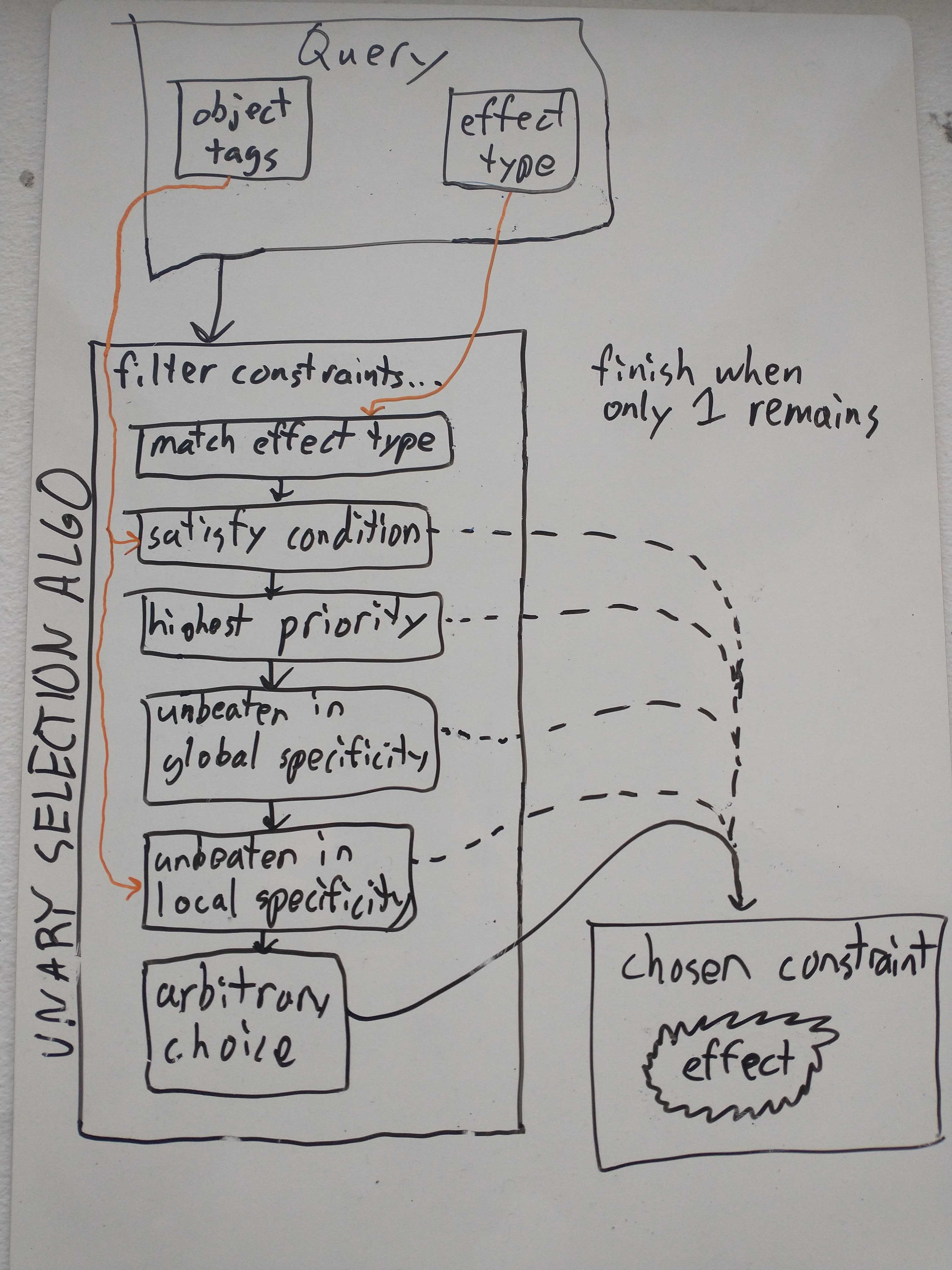
Match effect type. We begin with the set of all constraints in the design which have an effect whose type matches the query.
Condition Satisfaction. The constraint conditions must be satisfied. A constraint whose conditions are not satisfied will never be used, even if no alternative is available. A default value will be chosen instead. (In the case of
trace_widthandclearance, the default value is usually determined by theFabricationConstraintsused in the design.)Explicit priorities. Constraints with higher explicit priorities (set using the
prioritykeyword argument) are preferred. Higher numbers are higher priority, sopriority = 20will be preferred overpriority = 10. The default priority for constraints which don’t otherwise specify is zero. Negative priorities are allowed.Under ideal circumstances, explicit priority should not be needed — the specificity-based selection should handle most cases naturally. Priority is available as a fallback when you need to force a particular constraint to win, but using it disables the specificity principle for that priority level: a constraint at a higher priority will always beat a lower-priority constraint regardless of how specific its condition is.
As a filter, this step keeps all and only those constraints which are tied for the highest priority.
Global logical specificity. A constraint whose conditions are logically stronger is preferred. For example, a constraint with condition
Power() & IsViawill be preferred over simplyIsVia, because the property of both having the Power tag and being a via includes, tautologically, the property of being a via, but on the other hand, merely from the fact that an object is a via it does not necessarily follow that it has the Power tag. Note that logical strength here takes into account that child tags are considered (axiomatically) to imply their parent tags.One way of thinking about logical specificity is to imagine a hypothetical universe with objects of every possible combination of tags (provided such combinations always include parent tags). Then condition C is more logically specific than condition D if the set of objects satisfying C is a strict subset of the set of objects satisfying D. It is important that we consider all theoretically possible objects, though. For example,
Power() & IsViais stronger thanPower()because in theory an object could have thePower()tag but not be a via. The algorithm does not consider whether any such objects actually exist in the design.As a filter, this step discards all constraints for which there is another constraint which is globally more specific in this way. In other words all and only those constraints are kept which are unbeaten in global specificity.
Local logical specificity based on canonical tag order. Local specificity is similar to global specificity but it further considers the particular sets of tags possessed by the objects in question, in order. For example, a constraint with condition
IsVia & Power()will be preferred over a constraintIsCopper & Power() & MyTag()by a query on a via with bothPowerandMyTagapplied to it. This is because, even though neither of these logically implies the other in general (which would be global specificity), when the tags are considered in order,IsViacomes beforeMyTagin the canonical ordering and theIsVia & Power()condition is specific toIsViain the sense that it requires that tag to be present or else the condition would be false. In general, object type tags precede user tags in the canonical ordering; see that section for details.As a filter, this step walks through the query object’s tags in order and potentially discards constraints at every step. If some of the remaining constraints are specific to a given tag and others are not, when stepping through that tag, only the ones which are specific to that tag are kept.
Tie-breaking. If the above rules do not suffice to select a single constraint, the system applies additional tie-breaking heuristics based on the logical strength of the remaining constraints’ conditions (including negation). If these still do not resolve the tie, one of the remaining constraints will be selected deterministically but in a way that should not be relied upon.
Each step in this list acts as a filter to which constraints are considered at later steps; the process does not restart from scratch. As soon as only one constraint remains after a given filter, that is the constraint that will be chosen. (The exception is that it is always required for constraints to match the effect type and satisfy the conditions - if no constraint passes both of those filters, then no constraint will be chosen and a default value will be returned for the query.)
In general, constraints can have multiple effects if they are of different types; because constraint selection only ever occurs for one effect type at a time, this has no impact on the selection process.
Extended example#
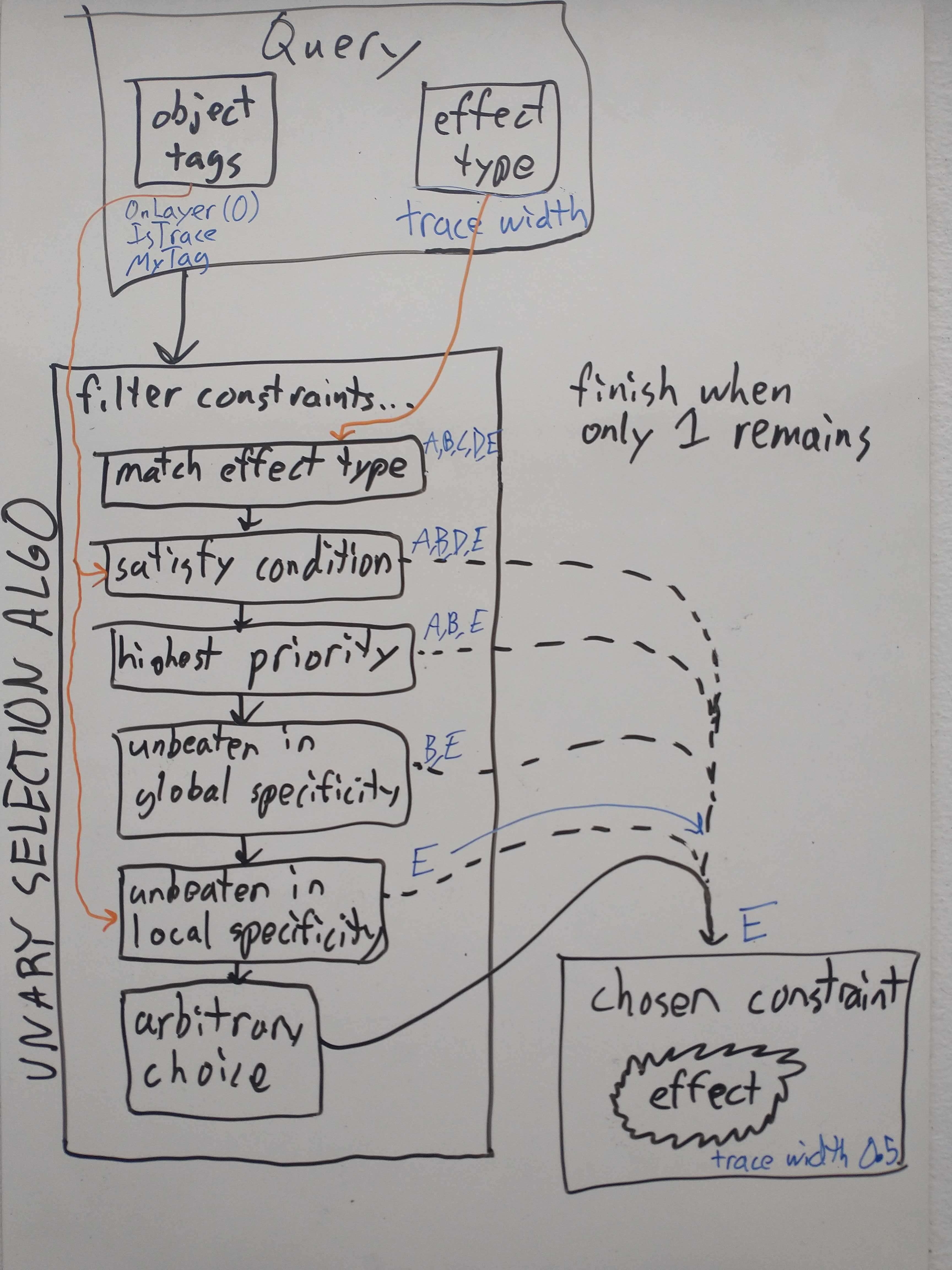
Suppose these are the only five constraints in the design with a trace_width
effect:
T = IsTrace
design_constraint(T).trace_width(0.1)                           # A
design_constraint(T & OnLayer(-1)).trace_width(0.2)             # B
design_constraint(T & OnLayer(0)).trace_width(0.3)              # C
design_constraint(T & OnLayer(-1) & MyTag(),
                  priority = -10).trace_width(0.4)              # D
design_constraint(T & MyTag()).trace_width(0.5)                 # E
Suppose that we are considering a trace on the bottom layer to which MyTag has
been applied.
Then the algorithm would run as follows:
Condition Satisfaction: Of the five, constraint C’s condition is not satisfied, so we throw out C.
Explicit priorities: Of A,B,D,E, all have priority 0 (by default) except for D, which has priority -10. 0 is greater than -10, so we throw out D.
Global specificity: Of A,B,E we see that B and E are logically incomparable, but both are stronger than A. So we throw out A.
Local specificity: For B and E we look at the object tags in order. E is more specific in having
MyTagwhereas B is more specific in havingOnLayer(-1). In the canonical tag ordering, user tags come before layer tags, because layer is considered a relatively more contextual piece of information to put in a condition. So E wins here.
Logical specificity - the core idea of constraint selection#
When a JITX design has many constraints and the system is being used as intended, logical specificity is the main principle which is used to filter constraints in practice. We saw this in our overview of the constraint selection algorithm, where the two main steps of the algorithm are the global and local versions of this principle respectively. (While explicit priorities can also be used to prefer some constraints over others, as discussed in the introduction, this is a blunt instrument because there is no way to make exceptions for special cases without tinkering with the entire setup.) In this section we will explain how the filtering steps for logical specificity work in greater technical detail.
Global logical specificity#
To understand precisely what it means for a constraint to be globally more
specific than another, imagine a hypothetical universe of objects with every
possible combination of tags. Then to say that a condition (boolean expression)
C is globally more specific than a condition D is simply to say that the set of
objects satisfying C is a strict subset of the set of objects satisfying D. We
may equally say that C implies D or that C is stronger than D. Returning to
our previous example, Power() & IsVia is logically more specific
(stronger) than IsVia because every object with both of these tags certainly
has the IsVia tag in particular, but also, an object may have only the IsVia
tag and not the Power tag.
We should clarify that what we mean by a possible object here is really just a
set of object tags which respects inheritance. In the parlance of logic, tags
correspond to variables, and possible objects correspond to truth assignments
with axioms corresponding to all the inheritance relations such as IsVia => IsCopper. So we could not have an object with just {IsVia, Power} as its set
of tags, but we could have {IsCopper, IsVia, Power}.
We should also emphasize that this universe of possible objects has nothing to
do with objects which actually exist in the design or which even could exist.
In our example it does not matter whether there is any via in the design which
does not have the Power tag - the system will always consider it possible
that such an object could exist. For another, less intuitive example, the
system considers it possible that an object has the Power tag but not the
IsCopper tag. See the section on best
practices for advice on how to avoid pitfalls
related to this. The only restriction on the sets of tags that the system
considers is that if it includes a tag it must also include its parent tags (and
their parent tags if any, etc.).
We gave an example where one constraint is indeed globally more specific than another. We should also give examples where this is not the case. Note that there are two basic ways that this can happen.
If one condition is
Power() & IsViaand the other isIsVia & MyTag(), then neither condition is more specific than the other. Obviously, it is possible to have vias withMyTagbut withoutPowerand vice versa. This is the most common reason why neither constraint would be more globally specific.If one condition is
(Power() | MyTag()) & IsViaand the other isIsVia & ~(~Power() & ~MyTag()), then both conditions imply the other. Exactly the same sets of objects satisfy these two conditions. SimilarlyIsCopper & IsViais exactly equivalent toIsVia, in view of the inheritance rules. In cases like these where conditions are logically equivalent, the system makes no distinction between the conditions at all, at any stage of the algorithm, which may lead to an arbitrary choice being made if these are the only constraints remaining from all other filters.
In typical usage there are many more than two constraints being considered at a time, so all of these relationships may occur simultaneously in the same set of constraints. The global specificity step of the selection algorithm filters out all constraints which are “unbeaten in global specificity”, i.e., all constraints such that there is no other constraint which is globally more specific. To illustrate this with a somewhat artificial example, suppose at this stage of the algorithm we encounter this set of conditions:
IsVia & Power() & MyTag()                (A)
MyTag() & Power() & IsCopper & IsVia     (B)
IsCopper & Power()                       (C)
IsCopper & MyTag()                       (D)
IsVia & MyChildTag()                     (E)
We can see that A is equivalent to B, both are more specific than either C or D, and neither A/B nor E is more specific than the other. The way the algorithm views this situation is that C and D are beaten, whereas A, B, and E are all unbeaten. Therefore A, B, and E are kept at this stage while C and D are discarded.
Local logical specificity#
Local logical specificity, like the global version of the principle, fundamentally relies on the logical content of the condition, i.e. what sets of tags make the condition true or false. Unlike global specificity however, the local specificity algorithm starts by considering the specific set of tags possessed by the actual object of the query. First we make a ordered list of these tags, and then we start stripping away the tags one at a time, always considering the effect this has on the truth or falsity of the condition.
The canonical tag ordering#
The local specificity starts with an ordered list of all the tags of the particular query object. However the ordering that is used to sort this list is defined globally. We call it the canonical tag ordering to emphasize that it never changes and is unaffected by how the constraints were written or any other design code. In particular it has nothing to do with the ordering in which tags appear in the conditions of individual constraints or the ordering which constraints appear in the code, both of which have no effect on the constraint selection algorithm.
Tags are processed in the following order (earlier tags are considered first and thus have higher priority in local specificity):
Object type tags, in the following order:
IsHole,IsNeckdown,IsThroughHole,IsBoardEdge,IsPad,IsVia,IsPour,IsTrace,IsCopper.User-defined tags, ordered alphabetically by name. (This ordering is an implementation detail and should not be relied upon.)
OnLayertags, in order of decreasing layer index, i.e., from bottom to top.
When the canonical tag ordering needs to be considered to determine specificity,
we make an ordered list (using the canonical ordering) of all the tags which
apply to the object in question. In cases of tag inheritance, the list only
contains tags which have no children that also apply. For example, if the list
includes MyChildTag it will not have MyTag. This also applies to the
conventional inheritance structure of implicit tags; for example if the list has
IsTrace it will not also have IsCopper.
How local logical specificity actually filters constraints#
The full procedure runs like this:
List all tags which apply to the object in their canonical ordering. We will work on a copy of this list called the working list.
Modify the working list by one step as follows. If the first tag in the list has parents, replace it by its parents, in canonical order. Otherwise, remove it from the list. Let’s call the tag that we just removed the active tag.
For each constraint which remains as a candidate, check the condition to see if it is specific to the active tag, meaning if removing the active tag from the full (unmodified) set of object tags would cause the condition to be no longer true.
If any constraints are specific to the active tag, then discard all constraints which are not specific to the active tag.
If there is only one constraint remaining, that constraint is chosen. Otherwise, return to step 2 and continue until a single constraint remains.
If the working tag list is exhausted and still multiple candidates remain, then local specificity has failed to choose a single constraint and the choice must be made arbitrarily.
Note that the accuracy of this description of the algorithm depends on certain mild assumptions on how disjunction and negation are used, which are explained in a later section. The design intent is that these assumptions are easily satisfied and you are unlikely to run into exceptional behavior by accident.
Local logical specificity: extended example#
Suppose we have these constraints:
class MyTag(Tag):
    pass
class MyChildTag(MyTag):
    pass

T = IsTrace
design_constraint(T & MyChildTag()).trace_width(0.1)               # A
design_constraint(T & IsNeckdown & ~OnLayer(0)).trace_width(0.2)   # B
design_constraint(T & OnLayer(-1) & IsNeckdown).trace_width(0.3)   # C
design_constraint(T & MyTag() & IsNeckdown).trace_width(0.4)       # D
design_constraint(T & OnLayer(-1) & MyTag()).trace_width(0.5)      # E
Further suppose we have a neckdown trace on bottom layer with the MyChildTag,
so all of these tags apply. Then the ordered tag list would be
IsNeckdown IsTrace MyChildTag OnLayer(-1)
(Note that MyTag and IsCopper do not appear in the list initially as they
are parents of other tags here.)
And the procedure would run as follows:
Remove
IsNeckdownfrom the list. Constraints B,C,D are specific to this tag whereas A and E are not, so A and E are discarded.Replace
IsTracebyIsCopper. This has no effect.Remove
IsCopperfrom the list. This has no effect.Replace
MyChildTagbyMyTag. This has no effect.Remove
MyTagfrom the list. Of the three remaining constraints, only constraint D is specific to MyTag, so D is the chosen constraint.
As another example, consider the same situation except the trace is not
neckdown. Then constraints B,C,D don’t apply at all (because their condition is
not satisfied), and the procedure would run until MyChildTag is replaced by
MyTag, at which point constraint E would be filtered out and constraint A is
chosen.
Avoiding pitfalls#
Correct use of disjunction and negation#
In an earlier section we described the detailed algorithm for how constraints are filtered for local logical specificity. The algorithm as described there is the intended behavior of the system, but it is theoretically possible to write some complicated constraint conditions that will cause the JITX backend to choose a different constraint. The main reason for this is that the backend uses an optimization involving disjunctive normal forms to speed up queries. By the design, the exceptional cases are rare and should not interfere with the functioning of a well-thought out set of constraints. To avoid exceptional behavior, it is sufficient to follow these restrictions when writing constraints:
When using negation, follow both of these principles:
Use negation only on individual tags (rather than larger sub-expressions).
Whenever negation is used, the negated tag should be conjoined with either a positive (not negated) tag or a disjunction of expressions each of which contains a positive tag.
Examples:
Good:
Power() & ~Power3V()negating a child tag as an exception to the parentGood:
~(OnLayer(0) | OnLayer(-1)) & IsTrace. Although this superficially violates the rule, it is equivalent to~OnLayer(0) & ~OnLayer(-1) & IsTracewhich is acceptable because of the positive tagIsTrace.Good:
~SpecialTag() & (NetTag1() | NetTag2() | NetTag3())Bad:
~NetTag1() & (Power() | ~SpecialTag())
When using disjunction, ensure at least one of the following is true:
The disjuncts (sub-expressions joined with
|) are mutually exclusive in practice. For exampleIsCopper | IsHoleorOnLayer(0) | OnLayer(-1). For this particular purpose, it does not matter whether it is logically possible for two disjuncts to be true simultaneously, only whether the design actually has an object which satisfies both.All of the disjuncts are user tags. Such as
Power() | SpecialTag(). The reason this specific case is okay is that the optimization would only change results up to reordering user tags, and the canonical ordering on user tags is unspecified anyway.
Note that if a condition does not use disjunction or negation, then these restrictions are satisfied vacuously so there is no problem. In general, if all of these restrictions are observed, then the algorithm steps given earlier are guaranteed to correctly predict the outcome.
Regarding the restriction on disjunction, there is actually a more general condition that ensures the algorithm behaves as expected:
Consider each variant of the entire condition obtained by choosing exactly one sub-expression in each disjunction, resulting in a disjunction-free expression. For any of these variants the effects of comparing local specificity against the condition of any other relevant constraint must be in agreement. The relevant constraints to compare are any whose conditions might be simultaneously satisfied in practice in the design. If more than one such constraint’s condition uses disjunction, then it is necessary to consider every possible combination of variants of these constraints (choosing one variant from each constraint) which can be simultaneously true.
However it is somewhat challenging to apply this in practice so we recommend sticking to the simpler rules.
Note that the exceptional behavior that can arise from violating these restrictions affects only the outcome of filtering for local specificity. It remains true that constraints which are globally more specific are always preferred.
Constraint selection for binary constraints#
So far we have described the selection algorithm as it applies to unary constraints. Binary constraints have some additional considerations. There are two basic issues:
What does the order of the two conditions mean?
How does the logical specificity principle apply when each constraint has two conditions?
In brief, the way the system addresses these issues is as follows:
By design, the order does not matter. If you switch the order of the conditions in any clearance constraint in the code, there will be no observable difference in behavior whatsoever.
Each binary constraint has its two conditions logically joined (“consolidated”) into a single condition. Then we use the same algorithm we have described in the unary case to select a constraint.
Both of these answers have caveats which we will explain. But let’s start by considering the easy case.
Binary conditions#
The basic idea for handling binary constraints is to refer back to the selection algorithm for unary constraints. We will do this by consolidating the two conditions of a binary constraint into a single condition.
The problem of consolidating conditions#
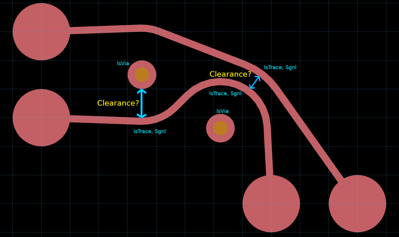
A naive way to do this would be to just combine them with & (logical-and).
But this does not make sense because it loses information about whether a tag
applies to both objects or only one. For example querying clearance from trace
to via is very different from clearance from trace to trace (as shown in
picture) and we would not want them to be confused.
Let’s look at exactly what goes wrong here. Suppose we have a constraint like this:
design_constraint(IsCopper & Sgnl(), IsVia).clearance(2.0)
The naive consolidated condition here would be IsCopper & Sgnl() & IsVia.
Since the Sgnl tag is only on the traces and not the vias, there is no object
in the picture which satisfies this condition. Thus it is unclear how we could
meaningfully apply the unary selection algorithm. Furthermore, if we consider
this alternative constraint:
design_constraint(IsCopper, IsVia & Sgnl()).clearance(2.0)
the consolidated condition would be exactly the same, even though as binary constraints these apply in quite different cases. For example, this one would apply between a signal via and a non-signal trace.
Consolidation of conditions#
Fundamentally to get a single condition that makes sense for a binary constraint
we need to recognize that there are two independent objects. Taking a second
look at the picture we see two
scenarios where clearance needs to be considered: one between two signal traces
and one between a signal trace and a via. We need to accurately reflect the
difference in meaning between saying one object has a certain tag, such as
Sgnl, and saying both objects do.
To accomplish this we conceptually duplicate all the tags. Let’s label the two
objects in question A and B. Now instead of the unary Sgnl tag we will have
both A-Sgnl and B-Sgnl tags, and similarly for every other tag.
Now we can consolidate the condition as follows:
A-IsCopper & A-Sgnl & B-IsVia
Similarly, if we have a constraint with disjunction like this:
design_constraint(IsTrace, IsHole | IsBoardEdge).clearance(0.5)
then the consolidated condition is
A-IsTrace & (B-IsHole | B-IsBoardEdge)
Now A-Sgnl & B-Sgnl would say both objects have the Sgnl tag, while A-Sgnl
would say only one of them does. But this leads to another problem: which
object is the A object and which is the B object?
Symmetrization of conditions#
Given that the two conditions of a clearance constraint may be quite different from each other, it obviously matters which condition is considered to apply to which object in any given physical situation. Unfortunately this choice is arbitrary in general. There is no principled way to decide which would apply to all pairs of objects in all circumstances. In view of this problem, the algorithm forcibly symmetrizes the consolidated condition. That is, the condition is rewritten so that the symmetrized condition is always satisfied if either one of the two possible orderings would have satisfied the original condition.
Formally, we start by making two different consolidated conditions, one for each ordering. So the symmetrized conditions in our previous two examples are as follows:
(A-IsCopper & A-Sgnl & B-IsVia) | (B-IsCopper & B-Sgnl & A-IsVia)
(A-IsTrace & (B-IsHole | B-IsBoardEdge)) | (B-IsTrace & (A-IsHole | A-IsBoardEdge))
These are the conditions we give as input to the usual unary constraint selection algorithm. Notice how this input would be unaffected (up to logical equivalence) if the order of the conditions in the original code were swapped.
Binary conditions and logical specificity#
Consolidating and symmetrizing binary conditions allows us to treat them as unary. You can tell if a binary constraint is more specific than another by applying the usual algorithm to the symmetrized consolidated versions of the conditions.
Note that for global specificity, intuitively it may be simpler to bypass this step and consider the binary conditions directly. The question is simply this: if you have two objects satisfying Condition 1 (in some order), does this logically force the same two objects to satisfy Condition 2 (in any order)?
For example, if you have these constraints:
design_constraint(IsVia & Sgnl(), IsVia).clearance(2.0)
design_constraint(IsCopper, IsCopper & Sgnl()).clearance(1.0)
we can see the first constraint is globally more specific than the second, because if you have a signal via and any other via, you tautologically also have a signal copper-object and another copper-object. We are in some sense “switching the order” of the conditions on the second constraint to see this, and that’s exactly what condition symmetrization entitles us to do.
Tag symmetrization#
By symmetrizing the conditions we have ensured that whether or not the constraint is applicable never depends on the choice of which object is which. Unfortunately, in some cases, we still have another asymmetry which would force us to make arbitrary choices. This comes up because of the local specificity principle and more specifically the canonical tag ordering.
The question is, how is the canonical tag ordering defined with respect to the duplicated tags?
The problem#
Unfortunately this situation actually presents a design dilemma insofar as there are common cases where the choice of canonical tag ordering here affects the outcome, effectively making an arbitrary choice that undermines our intention that it shouldn’t matter which order the conditions were written in.
To illustrate the problem, let’s consider a concrete example. Suppose you have these constraints:
design_constraint(IsCopper & Pwr(), IsCopper).clearance(1.5)
design_constraint(IsCopper & Sgnl(), IsCopper).clearance(1.0)
Assume Pwr and Sgnl are unrelated user tags that we have defined. Which
constraint will take effect when querying the clearance between a power trace
and a signal trace? The symmetrized consolidated conditions will be (after
simplifying the logical expressions):
A-IsCopper & B-IsCopper & (A-Pwr | B-Pwr)
A-IsCopper & B-IsCopper & (A-Sgnl | B-Sgnl)
Assuming neither Pwr nor Sgnl inherited from the other, neither of these is
globally more specific. What does the canonically-ordered tag list look like in
our scenario? We haven’t actually defined an ordering for the duplicated tags
but hypothetically it will look something like this:
B-IsTrace A-IsTrace B-Sgnl A-Pwr B-OnLayer(0) A-OnLayer(0)
The problem is that no matter what order we define on the duplicated tags, it is
fundamentally arbitrary whether A-Pwr comes before or after B-Sgnl in this
list. Because ultimately the choice of labels A and B is arbitrary. And
(unfortunately) the outcome of the constraint selection algorithm depends on the
choice. If B-Sgnl comes first, the constraint mentioning Sgnl will win so
the clearance is 1.0. If A-Pwr comes first, the other constraint will win and
set the clearance to 1.5.
The solution: merging clearance effects#
In view of the inherent arbitrariness here, the system has a special exceptional
behavior and takes the larger of the two clearances, which would be 1.5. The
way this merging behavior works is that we actually run the entire local
specificity algorithm twice using two different tag lists, one for both possible
object orderings (i.e. both choices of which object is A and which is B). Then
if (and only if) these give different results, we merge the results by taking
the higher clearance.
The order for duplicated tags is defined in a slightly complicated way, in order to ensure that the merging behavior is necessary only in cases where the arbitrary ordering of user tags affects the outcome. Basically for user tags we do all A tags first then all B tags. But for implicit tags we do the usual ordering as the primary sort, putting each A/B pair together.
The full local specificity algorithm for binary constraints#
In summary, here is the full procedure for constraint selection based on local specificity:
Consider both possible choices of which object is the A object and which is the B object. For each such ordering, create a separate tag list based on this canonical ordering:
All implicit tags which precede user tags, in their usual order. The usual canonical tag ordering is the primary sort, then A before B. (So for two traces, the ordering begins as
A-IsTrace B-IsTrace A-IsCopper B-IsCopper ...)All user tags for A.
All user tags for B.
All implicit tags which succeed user tags, in their usual order, similar to first step.
Apply the usual constraint selection algorithm for both of these tag lists. If they return the same constraint, that constraint is chosen. Otherwise, both constraints are chosen and the maximum clearance applies.
Detailed example#
Recall our example constraints from before:
design_constraint(IsCopper & Pwr(), IsCopper).clearance(1.5)
design_constraint(IsCopper & Sgnl(), IsCopper).clearance(1.0)
The symmetrized consolidated conditions are:
A-IsCopper & B-IsCopper & (A-Pwr | B-Pwr)
A-IsCopper & B-IsCopper & (A-Sgnl | B-Sgnl)
The canonically ordered tag lists are:
A-IsTrace B-IsTrace    A-Pwr B-Sgnl   A-OnLayer(0) B-OnLayer(0)
A-IsTrace B-IsTrace    A-Sgnl B-Pwr   A-OnLayer(0) B-OnLayer(0)
Now let’s run the local specificity algorithm in parallel for these two lists, taking note when something different happens:
Replace
A-IsTraceby parentA-IsCopper. Nothing happens.Drop
A-IsCopper. Both constraints are specific so we continue.Replace
B-IsTraceby parentB-IsCopper. Nothing happens.Drop
B-IsCopper. Again both constraints are specific so we continue.The next step depends on which ordering we chose.
Scenario 1: A is the power trace. The next tag to drop is
A-Pwr. The first constraint is specific but the second one is not. So the first constraint is chosen.Scenario 2: A is the signal trace. The next tag to drop is
A-Sgnl. The second constraint is specific but the first constraint is not, mirroring the previous scenario. So the second constraint is chosen.
Because two different constraints were chosen, the two results are merged, so we take the maximum clearance of 1.5.
Example where merging does not happen#
Let’s consider another example which is similar to the previous one but with some modifications:
the signal constraint also requires the trace to be neckdown
the signal trace is also neckdown
the power constraint also requires the traces to have an extra user tag
MyTagboth traces also have
MyTag
The constraints are:
design_constraint(IsCopper & Sgnl() & IsNeckdown, IsCopper).clearance(1.5)
design_constraint(IsCopper & Pwr() & MyTag(), IsCopper).clearance(1.0)
The symmetrized consolidated conditions are:
A-IsCopper & B-IsCopper & ((A-Sgnl & A-Neckdown) | (B-Sgnl & B-Neckdown))
A-IsCopper & B-IsCopper & ((A-Pwr & A-MyTag) | (B-Pwr & B-MyTag))
The two possible tag lists now look like this (noting that only the signal trace is neckdown):
A-IsNeckdown A-IsTrace B-IsTrace    A-Sgnl A-MyTag B-MyTag B-Pwr
B-IsNeckdown A-IsTrace B-IsTrace    A-MyTag A-Pwr B-Sgnl B-MyTag
(We have omitted the OnLayer(0) tags at the end for brevity; they do not
affect anything relevant to the discussion.)
Local specificity is again needed to determine the outcome. When we run local specificity, we get different behavior immediately because the first tag in the list is different.
Scenario 1: The first tag in the list is
A-IsNeckdown. The signal constraint is specific for this tag - it is untrue without it - whereas the power constraint is not. So the signal constraint is selected.Scenario 2: The first tag in the list is
B-IsNeckdown. The signal constraint again is specific for this tag, whereas the power constraint is not. So the signal constraint is selected.
Because the same constraint is selected in both cases, no merging happens and the clearance will be 1.0.
This example illustrates the general point that the merging will only happen if the arbitrary ordering of user tags is forced to matter. Here there is a difference in specificity with respect to an object type tag. This takes precedence and there is a clear and consistent choice of which constraint should be preferred according to the same principles outlined in the discussion of unary constraints.
Binary constraints other than clearance?#
Currently the only binary constraint effect type is clearance. We have explained how the algorithm is modified in two kinds of ways for these constraints:
symmetrization, which includes both:
The reasons for these are different. Consolidation serves to enable using the unary constraint algorithm applicable to binary constraints, so that it isn’t necessary to invent a completely separate algorithm. This is a pragmatic simplification which doesn’t inherently have any effect on behavior. On the other hand, symmetrization (of both conditions and tag lists) is necessary in some form to make the system behavior coherent and predictable for an effect type where you inherently cannot tell the difference between applying the effect in one order vs. another.
Conceivably in the future there may be binary effect types which are not symmetric in the way that clearance is. It would then make sense to apply consolidation to those constraints but not symmetrization. If applying the constraint for A,B does something observably different and independent from applying it to B,A, then obviously it should matter in which order you write the conditions.
Conclusion#
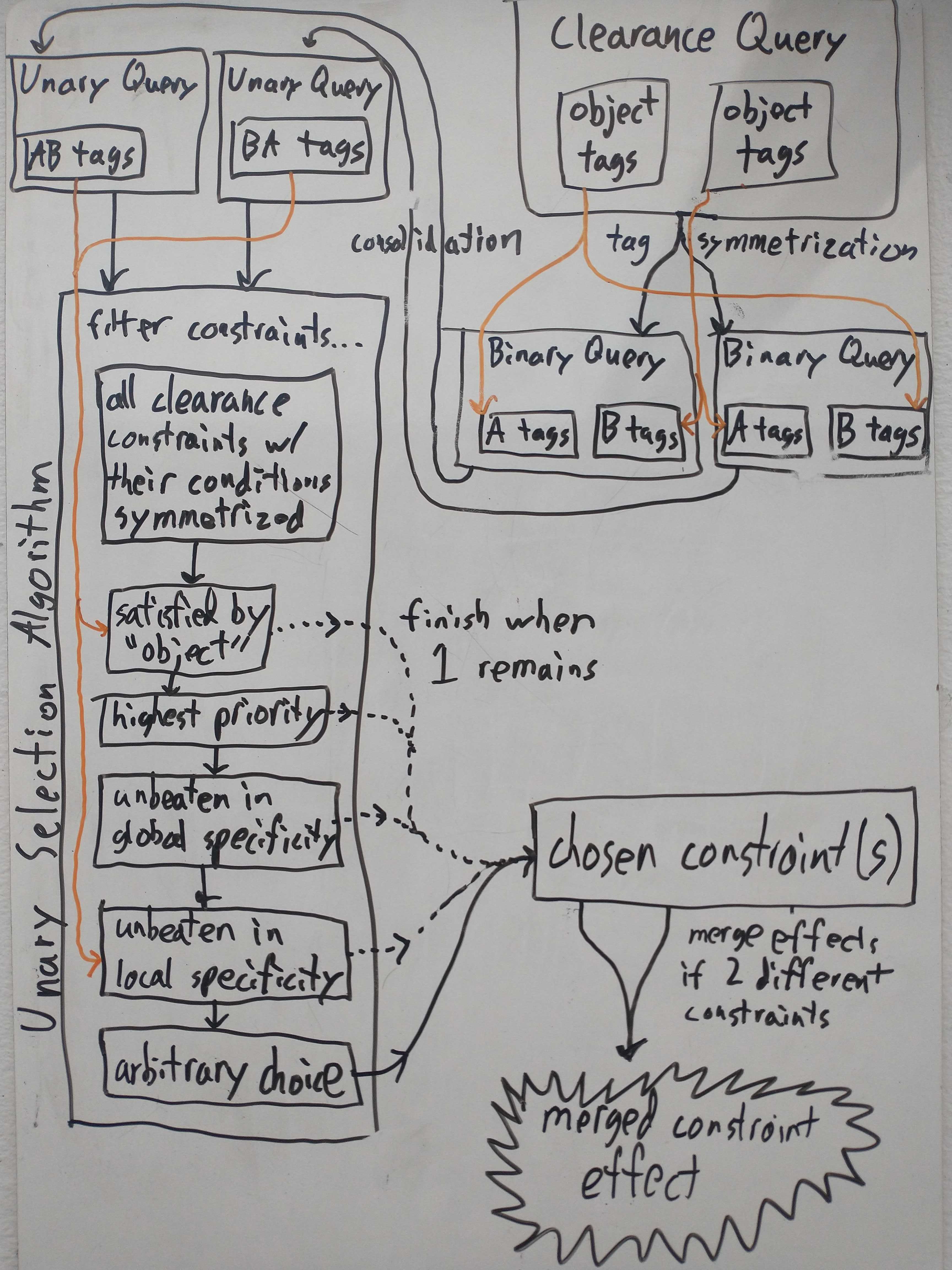
This diagram shows how all the pieces fit together. Starting with a clearance query, we apply tag symmetrization to effectively get two different queries which have the two different possible A/B labelings. This effectively puts us in two parallel worlds which don’t interact again until the very end. Consolidation then turns each of these into a unary query. We then run the unary selection algorithm on each of these queries. Note that in the selection algorithm we treat clearance constraints as unary constraints by symmetrizing their conditions. If the two chosen constraints are different, we merge their effects, i.e., take the maximum clearance.
In this diagram we have assumed that we have a clearance query as this is the only kind of binary constraint effect that exists currently. However a hypothetical future binary effect would likely work similarly, except that it may or may not use symmetrization.